
We now considered sources of error which may arise in our determination of
 through inaccuracies in our model.
We know from X-ray observations that, on large scales, the intra-cluster gas is typically very close to being isothermal out to radii of 750 kpc (Mushotsky (1996)). However, X-ray observations are insensitive to the low density gas far from the cluster centre (see equation 2), and so do not give us information on the temperature distribution of ``halo'' gas surrounding the central region.
If the temperature and density of the halo change in a manner such that the gas
remains in hydrostatic equilibrium with the central region, then the line of
sight pressure integral will be identical to that predicted by a purely
isothermal King model. Thus the S--Z effect will be exactly that predicted by
our simulations, and we will correctly estimate  .
.
We have performed simulations to quantify the effect of hydrostatic equilibrium
not being preserved in a gas halo. In one extreme example we assume that the
gas density is unchanged from that predicted by the King
model (equation 4) but allow the temperature to increase steadily
to 3 times its central value beyond a radius of 750 kpc. Although this
increases the temperature decrement which would be observed by a single dish
telescope by  , the S--Z flux that we would measure with the RT shortest
baselines would change by only
, the S--Z flux that we would measure with the RT shortest
baselines would change by only  . The reason for this is that the RT is an
interferometer and so resolves out any structure much larger than its
synthesised beam, such as the changes in the line of sight pressure integral
due to gas halos.
. The reason for this is that the RT is an
interferometer and so resolves out any structure much larger than its
synthesised beam, such as the changes in the line of sight pressure integral
due to gas halos.
We therefore conclude that the exact nature of the outer regions of the
intracluster gas does not significantly affect our  determinations.
In many clusters the gas density is sufficiently high at the centre that the radiative cooling time is less than the age of the cluster (Fabian et al. (1991)). To maintain pressure balance, this cool gas collapses inwards and becomes denser. These cooling flows have now been detected in most rich clusters through the greatly increased X-ray emission of the cool, dense, central gas.
The cooling flow radius is typically of the order of 100 kpc; outside this
region the gas remains isothermal. We therefore blank the pixels at the centre
of the X-ray map and fit an isothermal model to only the regions where there
has not been any significant cooling. If quasi-hydrostatic equilibrium is
maintained in the central regions where cooling flows are formed, then through
similar arguments to those used in section 4.1, the magnitude of the
S-Z effect in such a cluster is identical to that predicted by a purely
isothermal model. Thus we will be able to accurately estimate  in clusters
with quasi-hydrostatic cooling flows. Further, we have performed simulations
with worst-case, non-hydrostatic cooling flow models which indicate that even
in these clusters the effect on the expected flux measured by the RT would be
negligible.
in clusters
with quasi-hydrostatic cooling flows. Further, we have performed simulations
with worst-case, non-hydrostatic cooling flow models which indicate that even
in these clusters the effect on the expected flux measured by the RT would be
negligible.
It is possible that although clusters appear to be isothermal on large scales,
there may be temperature structure on small scales, below the resolution of
X-ray telescopes; the intracluster medium may consist of a mixture of cold,
dense and hot, diffuse clumps, still in hydrostatic equilibrium, and with
thermal conduction suppressed by magnetic fields. Modelling such a cluster
assuming that it was isothermal would incorrectly estimate both the gas
temperature and the X-ray surface brightness. However, these two errors tend to
cancel each other when calculating  . Using a simple two-phase model of a
clumped cluster where a volume fraction
. Using a simple two-phase model of a
clumped cluster where a volume fraction  has density
  and the
remaining
and the
remaining  has density 1, we find that the fractional error in
 resulting from modelling the cluster as being isothermal is given by
Thus for a cluster where half the gas volume has double the
temperature of the other half ( ), the error in
estimating
), the error in
estimating  is
is  . An extreme case where a tenth of the gas mass
occupies only a hundredth of the volume (
. An extreme case where a tenth of the gas mass
occupies only a hundredth of the volume ( ) leads to
a
) leads to
a  error; higher levels of clumping than given in this model could easily
be detected from the cluster's X-ray spectrum (Edge, private communication).
error; higher levels of clumping than given in this model could easily
be detected from the cluster's X-ray spectrum (Edge, private communication).
In calculating  we have assumed that the line of sight depth,
  ,
through the cluster is equal to the width in the plane of the
sky,
,
through the cluster is equal to the width in the plane of the
sky,  . If this is not the case then the calculated value of
Hubble's constant,
. If this is not the case then the calculated value of
Hubble's constant,  will be related to its real value by

X-ray maps show that clusters are elliptical in the plane of the sky, with
ellipticities of  being common. Therefore to obtain a robust estimate of
 we must observe an orientation-unbiased sample of clusters. This sample
can be compiled from a X-ray catalogue by selecting clusters above a certain
luminosity limit (rather than a surface brightness limit). At
present we are working on such a sample derived from the ROSAT All Sky Survey.
The true value of
we must observe an orientation-unbiased sample of clusters. This sample
can be compiled from a X-ray catalogue by selecting clusters above a certain
luminosity limit (rather than a surface brightness limit). At
present we are working on such a sample derived from the ROSAT All Sky Survey.
The true value of  is then the geometric mean of the individual estimates.
Combining X-ray and S--Z data depends on the cosmological deceleration
parameter  as well as
  (equation 3 assumes that
 ). In theory, observing two clusters will yield both of these
parameters. We have estimated the possible error in calculating
). In theory, observing two clusters will yield both of these
parameters. We have estimated the possible error in calculating  from
assuming that
from
assuming that  by simulating the response of the RT to a rich cluster
(
by simulating the response of the RT to a rich cluster
( ;
;  ;
;  ;
;  ) at redshifts between 0.1 and 10 for
  and 0.5. The results are
plotted in Figure 4.
and 0.5. The results are
plotted in Figure 4.
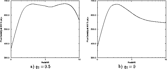
Figure 4: Predicted S--Z flux density on RT shortest
baseline when observing a rich cluster with  for different values of
the cosmological deceleration parameter,
for different values of
the cosmological deceleration parameter,  .
.
It can be seen that the value of  adopted makes little difference to the
predicted flux observed by the RT, especially between redshifts of 0.1 and 0.5.
It is also interesting to note that Figure 4 implies that if rich
clusters exist in the early universe, then we should be able to detect them
with the RT out to redshifts of 10.
adopted makes little difference to the
predicted flux observed by the RT, especially between redshifts of 0.1 and 0.5.
It is also interesting to note that Figure 4 implies that if rich
clusters exist in the early universe, then we should be able to detect them
with the RT out to redshifts of 10.  will, however, affect our fit to the
X-ray emission from the cluster. We calculate that at
will, however, affect our fit to the
X-ray emission from the cluster. We calculate that at  the change in
our estimate of
the change in
our estimate of  between assuming
  and
and  is only
  . The
error rises to
. The
error rises to  for a cluster at
  and to
  at
at  .
.