For this paper: postscript 1 Introduction... Abstract... 3 Application to simulated ...

2 Simulated Planck Surveyor observations  

In order to create simulated Planck Surveyor observations, we must first build a realistic model of the sky at each of the proposed observing frequencies. As mentioned above, dust, free--free and synchrotron emission from our own Galaxy, extragalactic radiosources and infrared galaxies, and the kinetic and thermal SZ effect from clusters of galaxies all contribute to sky emission at least at some frequencies and angular resolutions of interest. We assume that point sources may be removed as described above, and that the residual background of unsubtracted sources is negligible. Thus the simulations presented here include emission from the three Galactic components, the two SZ effects and the primordial CMBR fluctuations.

Simulated maps of these six components are constructed on -degree fields with 1.5 arcmin pixels; thus each map consists of pixels. A detailed discussion of these simulations is given by Bouchet et al. (1997) and Gispert & Bouchet (1997). The primary CMBR fluctuations are a realisation of strings produced by Francois Bouchet (Hobson et al. (1998) present the results for a COBE normalised CDM realisation of the CMB). Realisations of the kinetic and thermal SZ effects are generated using the Press-Schechter formalism, as discussed in Bouchet et al. (1997), which yields the number density of clusters per unit redshift, solid angle and flux density interval. The gas profiles of individual clusters are taken as King models, and their peculiar radial velocities are drawn at random from an assumed Gaussian velocity distribution with a standard deviation at of .

For the Galactic dust and free--free emission, IRAS maps are used as spatial templates. Comparison of dust, free--free and 21cm HI emission suggests the existence of a spatial correlation between these components (Kogut et al. (1996); Boulanger et al. (1996). In order to take account of these correlations, the simulations assume the existence of an HI-correlated component that accounts for 50 per cent of the free--free emission and 95 per cent of the dust emission. The remaining free--free and dust emission is assumed to come from a second, HI-uncorrelated component. For any particular simulation, a given IRAS map is used as a spatial template for the HI-correlated component and a contiguous map is used for the HI-uncorrelated component. The dust spectral behaviour is modelled as a single temperature component at 18 K with dust emissivity ; the rms level of fluctuations at any given frequency is scaled accordingly from the IRAS map. The IRAS map used here has an rms level approximately equal to the median level for such maps, i.e. about one-half of IRAS maps of this size have a lower rms, and half have a higher rms. The free--free intensity is assumed to vary as , and is normalised to give an rms temperature fluctuation of at 53 GHz.

No spatial template is available for the synchrotron emission at a sufficiently high angular resolution, so the simulations of this component are performed using the 408 MHz radio maps of Haslam et al. (1982), which have a resolution of 0.85 degrees, and adding to them small scale structure that follows a power spectrum. The synchrotron intensity is assumed vary as and its normalisation taken directly from the 408 MHz maps.

 
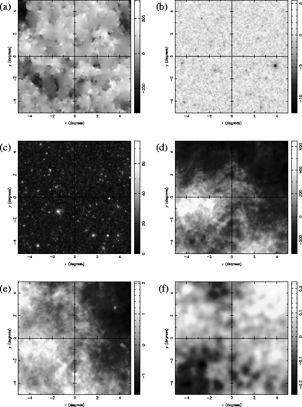
Figure 1: The -degree realisations of the six input components used to make simulated Planck Surveyor observations: (a) primary CMBR fluctuations; (b) kinetic SZ effect; (c) thermal SZ effect; (d) Galactic dust; (e) Galactic free--free; (d) Galactic synchrotron emission. Each component is plotted at 300 GHz and has been convolved with a Gaussian beam of FWHM equal to 4.5 arcmin, the maximum angular resolution proposed for the Planck Surveyor. The map units are equivalent thermodynamic temperature in . 

For primary CMBR fluctuations it is usual to work in terms of temperature rather than intensity. A temperature difference on the sky leads to a fluctuation in the intensity given by

where is the Planck function and is the mean temperature of the CMBR (Mather et al. (1994)). The conversion factor can be approximated by

where . In order to compare the relative level of fluctuations in each physical component we shall adopt the convention of Tegmark & Efstathiou (1996) and also define the equivalent thermodynamic temperature fluctuation for the other components by

where denotes the relevant physical foreground component. We note that, in general, the `temperature' fluctuations of these other components will be frequency dependent, unlike those of the CMBR. For the remainder of this paper, fluctuations will be quoted in temperature units measured in .

The realisations of the six input components used to make simulated observations are shown in Fig. 1. Each component is plotted at 300 GHz and, for illustration purposes, has been convolved with a Gaussian beam of FWHM equal to 4.5 arcmin, which is the highest angular resolution proposed for the Planck Surveyor. For convenience, we have also set the mean of each map to zero, in order to highlight the relative level of fluctuations due to each component.

From Fig. 1 we see that, as expected, the emission due to primordial CMBR fluctuations appears non-Gaussian in nature. This is, of course, a direct consequence of using a topological defect model to create this realisation. If the CMBR realisation were instead created assuming an alternative theory of structure formation such as standard CDM, for example, then the CMBR fluctuations are required to be Gaussian, and will not exhibit sharp edges. The emission due to the kinetic and thermal SZ effects is clearly highly non-Gaussian, being dominated by resolved and unresolved clusters that appears as sharp peaks of emission. As we would expect, although an obvious correlation exists between the positions of the kinetic and thermal SZ effects, the signs and magnitudes of the kinetic effect are not correlated with those of the thermal effect. We also note that the IRAS maps used as templates for the Galactic dust and free--free emission also appear quite non-Gaussian; the imposed correlation between the dust and free--free emission is also clearly seen. Finally, the synchrotron emission seems quite Gaussian, although this appearance is due mainly to the addition to the Haslam 408 MHz map of Gaussian small scale structure, following a power law, on angular scales below 0.85 degrees.

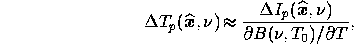
The azimuthally-averaged power spectra of the input maps are shown in Fig. 2. At lower multipoles, all three Galactic components have power spectra which vary roughly as (for the synchrotron component small scale structure with this power spectrum was added artificially for ). For the kinetic and thermal SZ effects, however, the power spectra are quite different and are better approximated by a white-noise power spectrum , as expected for Poisson-distributed processes.

 
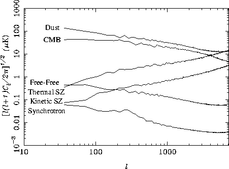
Figure 2: The azimuthally-averaged power spectra of the input maps at 300 GHz. 

 
Figure 3: The rms thermodynamic temperature fluctuations at the Planck Surveyor observing frequencies due to each physical component, after convolution with the appropriate beam and using a sampling rate of FWHM/2.4. The rms noise per pixel at each frequency channel is also plotted. 

Using the realisations for each physical component shown in Fig. 1, it is straightforward to simulate Planck Surveyor observations. The experiment consists of two mains parts: the Low Frequency Instrument (LFI), which uses HEMT radio receivers, and the High Frequency Instrument (HFI), which contains bolometer arrays. Since the final design of the satellite is still undecided, the precise values of observational parameters for the LFI and HFI are subject to revision. Nevertheless, recent proposed changes to both instruments may significantly improve the sensitivity of the satellite, as compared to the design outlined in the ESA phase A study (Bersanelli et al. (1996)). Therefore, although these modifications are not yet finalised, we have incorporated the latest design specifications into our simulations. The parameters used in making the simulated observations are given in Table 1 (Efstathiou, private communication).

 
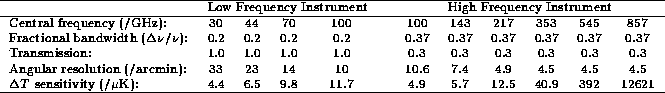
Table 1: Proposed observational parameters for the Planck Surveyor satellite (Efstathiou, private communication). Angular resolution is quoted as FWHM for a Gaussian beam. Sensitivities are quoted per FWHM for 12 months of observation. 

The simulated observations are produced by integrating the emission due to each physical component across each waveband, assuming the transmission is uniform across the band. At each observing frequency, the total sky emission is convolved with a Gaussian beam of the appropriate FWHM. Finally, isotropic noise is added to the maps, assuming a spatial sampling rate of FWHM/2.4 at each frequency. We note, however, that the assumption of isotropic noise is not required by the separation algorithms discussed in the companion paper. We have also assumed that any striping due to the scanning strategy and noise has been removed to sufficient accuracy that any residuals are negligible.

Fig. 3 shows the rms temperature fluctuations as a function of observing frequency due to each physical component, after convolution with the appropriate beam. The rms noise per pixel at each frequency channel is also plotted. We see from the figure that, as expected, the rms temperature fluctuation of the CMBR is almost constant across the frequency channels, the only variation being due to the convolution with beams of different sizes. Furthermore, for all channels up to 217 GHz, the CMBR signal is several times the level of the instrumental noise. At higher frequencies, the noise level exceeds the CMBR signal but is itself dominated by Galactic dust emission. We also see a sharp dip in the rms level of the thermal SZ effect at 217 GHz, since the emission from this component is close to zero at this frequency. At any given frequency, the rms level of the thermal SZ effect is at least an order of magnitude below that of the dominant component. The kinetic SZ effect has the same spectral characteristics as the CMBR, but the effect of convolution with beams of different sizes has a significant effect on the point-like emission and leads to a more pronounced variation in the observed rms level than for the CMBR. The observed rms level of the kinetic SZ is at least two orders of magnitude below the dominant component at any given frequency. In a similar manner, the Galactic free--free and synchrotron emission are also completely dominated by either CMBR or dust emission at all observing frequencies.

The observed maps at each of the ten Planck Surveyor frequencies are shown in Fig. 4 in units of equivalent thermodynamic temperature measured in K.

 
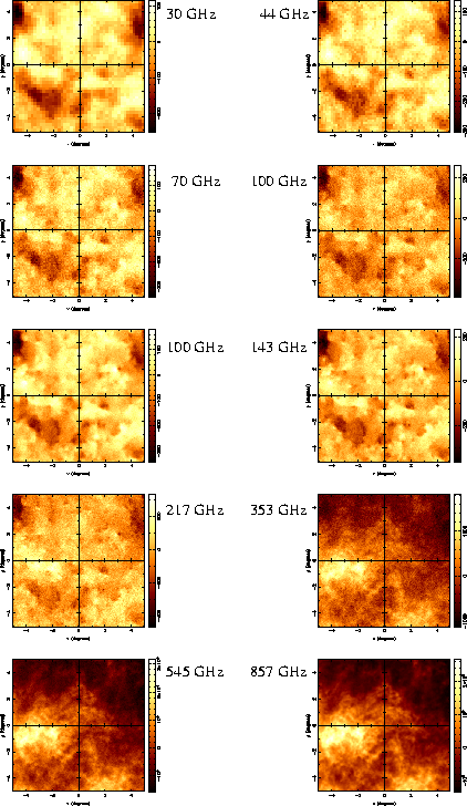
Figure 4: The -degree maps observed at each of the ten Planck Surveyor frequencies listed in Table 1. At each frequency we assume a Gaussian beam with the appropriate FWHM and a sampling rate of FWHM/2.4. Isotropic noise with the relevant rms has been added to each map. The map units are equivalent thermodynamic temperature in . 

The coarse pixelisation at the lower observing frequencies is due to the FWHM/2.4 sampling rate. Moreover, at these lower frequencies, the effect of convolution with the relatively large beam is also easily seen. As the observing frequency increases, the beam size becomes smaller, leading to a corresponding increase in the sampling rate. Consequently, the observed maps more closely resemble the input map of the dominant physical component at each frequency. As may have been anticipated from Fig. 3, the emission in the lowest seven channels is dominated by the CMBR, whereas dust emission dominates in the highest three channels. Indeed, the main reason for the inclusion of the highest frequency channels is to obtain an accurate dust model, in order that it may be subtracted from lower frequency channels with some confidence. Perhaps the most notable feature of the ten channels maps is that, at least by eye, it is not possible to discern features due to physical components other than the CMBR or dust.