Small fluctuations in each of the terms  ,
,  ,
,  ,
,  ,
,
 and
and  (generically denoted as
  ) appearing in equation 2
will lead to a change in the observed signal which can mimic a true sky
fluctuation
) appearing in equation 2
will lead to a change in the observed signal which can mimic a true sky
fluctuation  according to:
The results of section 2 can be used to calculate the susceptibility of the radiometer to each source of spurious fluctuation.
In this section, we will calculate the change in the output signal for a small
change in the noise temperature of one of the amplifiers. We start with
equation 2, let  , and then consider the derivative of
the output with respect to
, and then consider the derivative of
the output with respect to  :
:
Note that:
Putting these together, one finds that a change in amplifier noise temperature,
 can mimic a change in input signal,
  .
Incorporating the fact that both amplifiers (which have uncorrelated noise) can
contribute increases this effect by
.
Incorporating the fact that both amplifiers (which have uncorrelated noise) can
contribute increases this effect by  (this is equivalent to adding
the two contributions in quadrature). The result is:
(this is equivalent to adding
the two contributions in quadrature). The result is:
If the reference load is at the same temperature as the sky, then  (no DC
gain difference) and there is no effect to worry about. As
(no DC
gain difference) and there is no effect to worry about. As  departs from 1
the effect is of more concern.
departs from 1
the effect is of more concern.
Given this, we must now calculate the post-detection frequency,  , at which
the contributions from gain fluctuations are equal to the white noise from an
ideal radiometer:
, at which
the contributions from gain fluctuations are equal to the white noise from an
ideal radiometer:
The ideal sensitivity of the radiometer is (see the Seiffert et al. (1997) for a detailed discussion):
Substituting for the two sides of equation (13) one gets
Dividing each side by  and rearranging yields:
We will use  and
and  Hz. Finally, by using
equation 8 for the noise temperature fluctuations, we have the knee
frequency
Hz. Finally, by using
equation 8 for the noise temperature fluctuations, we have the knee
frequency
Assuming a 20% bandwidth for our frequency channels and an antenna temperature
 K, we tabulate the resulting knee frequencies in column 4 of Table
1 for several choices of
K, we tabulate the resulting knee frequencies in column 4 of Table
1 for several choices of  ,
,  and the corresponding
values of
and the corresponding
values of  .
.
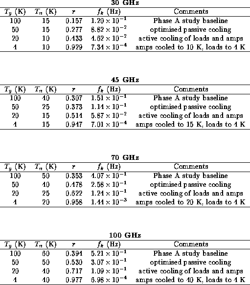
Table 1:  knee frequency for PLANCK LFI radiometers.
From equation 17 it results that that in the space  ,
,  ,
,  the curves of equal
  are hyperboles on any plane parallel to the plane
 ,
,  . Figure 2 shows several curves of equal
  for
the four considered frequencies. The knee frequency must be compared to the
spin frequency
for
the four considered frequencies. The knee frequency must be compared to the
spin frequency  ; for the PLANCK observational strategy
  r.p.m.,
i.e. 0.017 Hz.
r.p.m.,
i.e. 0.017 Hz.
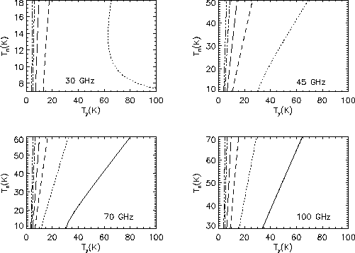
Figure 2: The curves of equal  on the plane
 ,
,  are plotted; an antenna temperature
  K is assumed. Each
panel refers to a different frequency channel (30, 45, 70 and 100 GHz). The
different lines refer to:
K is assumed. Each
panel refers to a different frequency channel (30, 45, 70 and 100 GHz). The
different lines refer to:  (Hz) = 0.3 (solid line), 0.1 (dotted line),
0.03 (dashed line), 0.01 (long dashes), 0.003 (dotted-dashed line), 0.001
(three dots-dashes). For the channels at 30 and 45 GHz the case
(Hz) = 0.3 (solid line), 0.1 (dotted line),
0.03 (dashed line), 0.01 (long dashes), 0.003 (dotted-dashed line), 0.001
(three dots-dashes). For the channels at 30 and 45 GHz the case  Hz
does not occur independently of cooling optimisation and is not reported.
Hz
does not occur independently of cooling optimisation and is not reported.
This radiometer is not sensitive to gain fluctuations in first order. We have indeed calculated how the output will change with respect to a small change in the gain of one of the amplifiers.
In the case  and by using the expression for
  , we have
obtained that the output change cancels completely. The conclusion is that, to
first order, gain fluctuations in the both amplifiers do not mimic a sky
signal fluctuation. We note that the second order cross terms are not zero, but
, we have
obtained that the output change cancels completely. The conclusion is that, to
first order, gain fluctuations in the both amplifiers do not mimic a sky
signal fluctuation. We note that the second order cross terms are not zero, but
 contribution is too small to be of concern here.
By carrying out analogous calculations, we derive the output changes mimicked by
reference load fluctuations and by fluctuations in  ; we find respectively:
 and
and  . Therefore they are equal to the white noise respectively for
 and
and  . In these cases the fluctuations in
  or
or  became
important.
became
important.
We have above discussed to what extent fluctuations in the different parts of
our radiometer can mimic true signal variations. A complete treatment of all
contributions together is quite difficult. On the other hand, under the
assumption that all fluctuations terms are uncorrelated, an estimate of their
global effect can be derived by comparing the change of  due to a true
sky temperature variation with the quadrature sum of the signal mimicked by the
different instrumental effects.
due to a true
sky temperature variation with the quadrature sum of the signal mimicked by the
different instrumental effects.
By using the above results, in the case  ,
,  ,
after algebraic manipulations we have:
,
after algebraic manipulations we have:
The basic information of the above equation was already implicit in the
equation 11 of Bersanelli et al. (1995), when  is derived from the condition
 (with the present notation for the
interesting quantities), and its fluctuations are obtained by the sum in
quadrature of the fluctuations of
(with the present notation for the
interesting quantities), and its fluctuations are obtained by the sum in
quadrature of the fluctuations of  ,
,  and
and  . We note that in
equation 18 the two terms related to the two amplifiers gain
fluctuations do not appear, because they are negligible at first order, as
previously discussed.
. We note that in
equation 18 the two terms related to the two amplifiers gain
fluctuations do not appear, because they are negligible at first order, as
previously discussed.
We can also see from this equation that the effect of white noise fluctuations
in  or
or  is to raise the overall white noise level, thereby lowering the
knee frequency (but decreasing the overall sensitivity). On the other hand the
limits on
is to raise the overall white noise level, thereby lowering the
knee frequency (but decreasing the overall sensitivity). On the other hand the
limits on  and
and  fluctuations given above can be realistically met with
present technology.
fluctuations given above can be realistically met with
present technology.
More generally, the fluctuations in  and
and  may have a complicated
spectral shape. In this case, a single knee frequency and white noise level
are an inadequate description of the noise; one must instead consider the shape
of the composite noise spectrum.
may have a complicated
spectral shape. In this case, a single knee frequency and white noise level
are an inadequate description of the noise; one must instead consider the shape
of the composite noise spectrum.


